

This guest post was co-authored by Ross Gore, Christopher J. Lynch, Craig Jordan, Virginia Zamponi, Kevin O’Brien, and Erik Jensen at the Virginia Modeling, Analysis & Simulation Center (VMASC).
Sensitivity analysis
Our story begins late at night wih a heroic researcher hard at work. Sat at their computer ahead of an important looming deadline, the researcher is busy analyzing the outcomes of various simulation runs. For some scenarios, the researcher’s simulation produces outcomes which match their expectations, but for others the results diverge dramatically.
This sort of experience will be recognizable to anybody who has constructed an even remotely complex model of the real world before. Under circumstances where it is infeasible or impractical to study a system directly, researchers develop simulations using HASH to emulate a system's inner workings. When the outputs of these simulations fail to match experimental data, or prevailing expert opinions, researchers are faced with solving a challenging problem: does the unexpected output reveal new knowledge about the system or is it due to a bug in code, incorrect data, or bad assumption? Without the ability to easily conduct sensitivity analyses, making this determination requires checking source code, reviewing data integrity, and unpicking the logic that powers simulations.
Motivated by the high cost and labor intensive nature of identifying conditions and source code statements that drive a simulation towards an unexpected output we have developed the VMASC Sensitivity Assessor, an online tool built to identify conditions and variables within HASH models that may consistently drive simulation runs towards unexpected outcomes.
In this post we'll explore how to download, process, and then analyze the outputs of HASH simulation model experiment runs. The data transformation and sensitivity analysis tools used in this post were developed at the Virginia Modeling, Analysis, and Simulation Center of Old Dominion University by members of the Data Analytics Working Group. These tools are public facing and free to use.
Making it real with an actual HASH simulation
We'll explore how the Sensitivity Assessor can be used to improve our understanding of disease transmission using an epidemiological HASH simulation model. Within our chosen simulation, agents are positioned randomly within the landscape. Some are initially ill; others are healthy but susceptible to illness. At each time step, agents move randomly throughout the simulated landscape. While moving randomly, if a healthy agent encounters an infected agent, the healthy agent becomes sick with a certain probability. When an agent becomes sick the agent is assigned a chance of recovery. Every sick agent increments their accumulated sick time at the start of each new time step. Once the sick time exceeds the sickness duration value, the agent either (i) dies (based on their chance of recovery) or (ii) survives and becomes immune. Once an agent becomes immune, the immunity lasts only for a specified number of time steps. Once the immunity period for an agent is reached, the agent returns to a healthy state but remains susceptible to illness.
The following figures show the HASH simulation as it progresses. Green squares represent the healthy agents, red squares represent the sick agents, and white squares represent the immune agents. The first screenshot displays the start of the simulation immediately following the initialization of all agents. The second figure shows the simulation after fifteen time steps and the third figure displays the simulation state after thirty time steps.

Figure 1: start of the simulation immediately following initialization

Figure 2: the state of the simulation after 15 time steps

Figure 3: the state of the simulation after 30 time steps
The simulation is meant to represent the spread of a virus and its effects on the population. However, there are times when the number of healthy agents within the simulation falls to zero depending on input values. Initially one may not anticipate that all agents in the simulation can become sick. This is an alarming outcome as it would imply that there are not any healthy people to provide healthcare or other essential services.
The following screen capture shows the graph of the infection process for one of the experiments that was created. It highlights a simulation run where the number of healthy agents falls to zero.
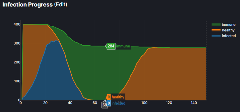
Figure 4: a times series of the immune, infected and healthy agents for a simulation run
As researchers we asked the question – “How can we better understand and quantify the dynamics related to the input parameters in the simulation that contribute to simulation runs with no healthy people in the population at a point in time?”
Later on in this post we apply the Sensitivity Assessor to explore this question. However, before we do so it is helpful to get a sense of what the Sensitivity Assessor is based on and what it can do for you (besides answering questions like this one in your HASH simulations).
What is the Sensitivity Assessor based on?
The goal of the Sensitivity Assessor is to take the ideas software engineers use to automatically identify the locations of bugs within programs and adapt them for researchers working with simulations. Specifically, there are a few main concepts behind the Sensitivity Assessor:
- Test writing — identifying if a simulation run produces the anticipated output or not. In software engineering a test case either passes or fails. In order to take advantage of automated debugging methods we need to identify if a simulation run produces the anticipated output or not. Similarly, it is important to keep in mind that the Sensitivity Assessor can only work if some runs produce the anticipated output while others do not. For cases where anticipated and unanticipated outcomes occur, the Sensitivity Assessor assists in identifying locations in the simulation that are likely contributing to these outcomes.
- Employing predicates — a predicate is a conditional proposition including at least one variable in a researcher’s HASH simulation that can be evaluated as either true or false. Predicates are a little easier to understand with examples:
x > 0is a predicate because it can be evaluated at a given point of time in the simulation as either true or falsey > zis a predicate because it can be evaluated at a given point of time in the simulation as either true or falsex > 0ANDy > zis a predicate because it can be evaluated at a given point of time in the simulation as either true or false4is not a predicate because it cannot be evaluated at a given point of time in the simulation as either true or falsexis a predicate if it reflects a boolean (true/false) value in the simulation. However, if it just reflects an integer or continuous number then it is not a predicate. This is because it cannot be evaluated at a given point of time in the simulation as either true or false.
- Predicates of many kinds — predicates can come in different “flavors and sizes”. An important thing to keep in mind when working with the Sensitivity Assessor is that there are multiple different ways to specify what types of predicates you want to be included. For example:
- The predicate
x > 0only contains one variable and it is compared to a number. Furthermore, we can specify the predicate without running the simulation (i.e. we don’t need to know every value thatxwill take on in the simulation before writing the predicate.). - The predicate
x > ycontains two variables and we can specify the predicate without running the simulation (i.e. we don’t need to know every value thatxorywill take on in the simulation before writing the predicate.) - The predicate
x > μx + σx(whereμxis the average value ofxandσxis the standard deviation in all the provided simulation runs) only contains one variable but requires having all the simulation runs complete to compute the values needed within the predicate (i.e.μxandσx). - The predicate
y > μx + σx(whereμxis the average value ofxandσxis the standard deviation in all the provided simulation runs) contains two variables and requires having all the simulation runs to compute the values needed within the predicate (i.e.μxandσx).
What can the Sensitivity Assessor do for me?
The Sensitivity Assessor (SA) provides new analytic and insight gathering capabilities for analyzing your HASH simulation outcomes. The SA allows you to build evidence to support interpretation and explanations of your models’ outcomes. A consistent set of capabilities for exploring data make the assessments reproducible, transparent, and easily shareable. Specifically, the Sensitivity Assessor helps in three ways:
1. Explore and sanity-check model variables
The Sensitivity Assessor provides data analysis capabilities that facilitate exploration and sanity checking of the variables from model inputs and outputs. A data description of each variable within the input file is provided using descriptive statistics. The goal is to provide insight into the central tendency of each variable (i.e., mean and median), the distribution around that tendency (i.e., standard deviation (SD) and median absolute deviation (MAD)), minimum (Min) and maximum (Max) values, and the number of samples (n).
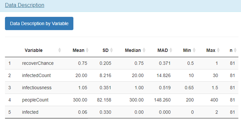
Figure 5: Sensitivity Assessor - Exploratory Data Analysis (EDA) capabilities
2. Verify requirements that should always hold
Simulations can frequently have a set of requirements that must always hold and can never be violated. Examples include some variable values: (1) always being positive, (2) not exceeding threshold values, or (3) being equal to some value.
The Sensitivity Assessor allows users to define requirements of the simulation that should always hold and never be violated. An intuitive interface exists for easily defining requirements in the form of different types of predicates. Variables are then read in from the simulation output, i.e., the input file, and these provide the variable names for building the predicates. The Sensitivity Assessor then scans simulation run outcomes and displays to users the number of times that a defined requirement appears within the simulation outputs, the number of times it is met, and the number of violations identified (if any).
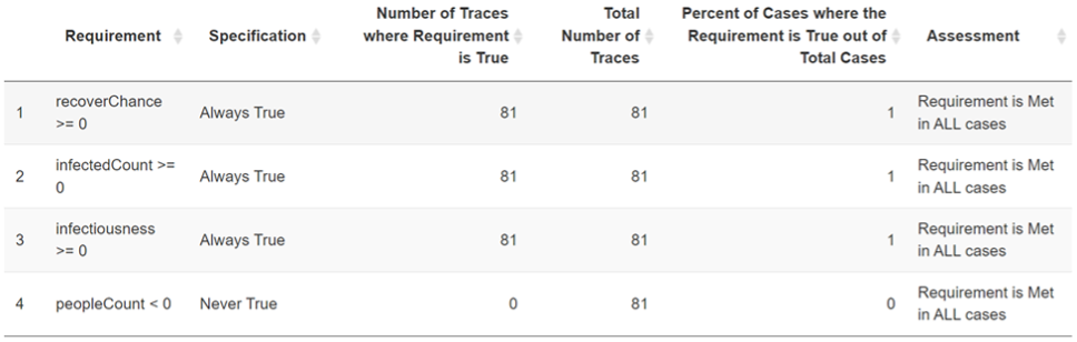
Figure 6: verifying requirements with the Sensitivity Assessor
A summary table provides details on the setup of the requirements and their resulting assessment, as follows:
- Requirement: reflects the user created requirement.
- Specification: whether the Requirement should always or never evaluate to true.
- Number of Traces where Requirement is True: the total times that the requirement evaluates true within the input file. Note that this does not take into account the assigned Specification.
- Total Number of Traces: the total number of lines in the input file.
- Percent of Cases where the Requirement is True out of Total Cases: this is the coverage of the Requirement within the input file. If a Requirement should always be true, then the number of cases where the Requirement evaluates true should equal the total number of cases. This would then result in a value of
1. However, if the Specification is set to Never True, then the Requirement should appear in no cases and the result should be a value of0. - Assessment: the proper interpretation of the result when accounting for both the Requirement and the Specification. As a result, percentages of both
0s and1s can be interpreted as successful, when appropriate, and are denoted as “Requirement is Met in ALL cases”.
3. Quantify to what extent certain conditions do or don't contribute to variables of interest
The Sensitivity Assessor quantifies the extent to which certain conditions contribute to the occurrence of a variable of interest. To facilitate this assessment, you must first specify which variable is of interest (this is done on the Explore Data tab immediately after uploading a file). Then, specify a range of interest for the variable of interest. This forms the feasible region for exploration. A slider bar exists on the “Assess Condition Sensitivity” tab to allow for specifying a desired range. The min and max values on the slider automatically update to reflect the range of values for the variable of interest from the input file. A range of interest must include at least one of the data points for the variable of interest and cannot include all of the data points for the variable of interest.
The sensitivity assessment is conducted using the variables and data provided to the Sensitivity Assessor. Data is expected to be in tidy with variables in each column and each row representing a set of observations of the variables. Assessments are conducted with respect to the specified variable of interest within the range of interest that is specified using the slider bars.
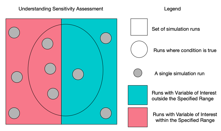
Figure 7: understanding the quantification of a sensitivity assessment
The remaining variables are used to form conditions. These conditions are evaluated using every row of the input file and the total number of times that the condition evaluates true is compared against the total number of rows in the input file. Specifically, the following definitions are used to provide insight into the data through our sensitivity assessment metric:
- Condition: a predicate to explore within the simulation output. Constructed using variables from the input file that have not been selected as the variable of interest.
- Number of Traces where the Condition is True: the number of times that the condition evaluates true within the input file. This is conducted by looking at each observation (i.e., row) within the file that contains the relevant variable(s) and assessing if the condition holds or not.
- Total Number of Traces: the total number of rows (i.e., observations per variable) in the input file.
- Likelihood that the Condition appears alongside Assessment Variable and Range –
Likelihood_1: a correlation measure that explores the likelihood that the condition appears alongside the specified range for the variable of interest. Note that the specified range for the variable of interest remains constant across the entire set of checks, so all checks are conducted against the same target. The following equation conveysLikelihood_1:

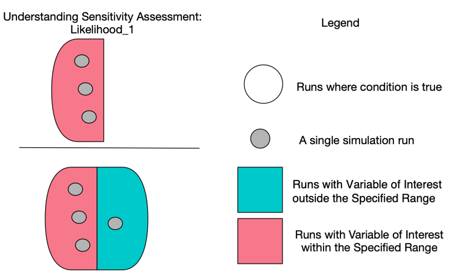
Figure 8: understanding Likelihood_1
- Likelihood that the Condition appears alongside Assessment Variable and Range –
Likelihood_2: a measure of how often the Condition is True at the same time that the variable of interest is within its specified range of interest. The following equation conveysLikelihood_2:

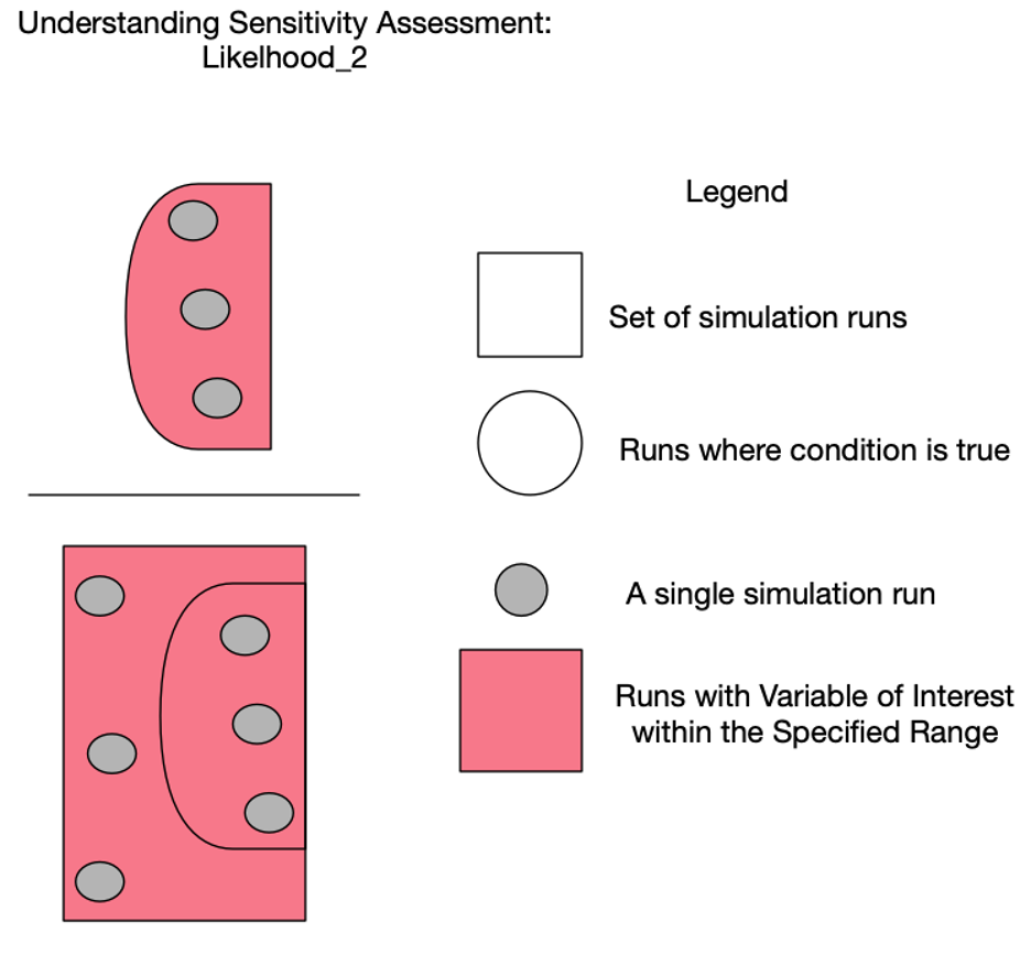
Figure 9: understanding Likelihood_2
- Sensitivity Assessment: the harmonic mean of
Likelihood_1andLikelihood_2. This measure is used for ranking the conditions contributing to the variable of interest within its specified range.- The following equation conveys the
Sensitivity Assessment.

- The outcomes from the sensitivity assessment are tabulated into a visually explorable table that conveys each of the above metrics. The table provides transparency from the
Sensitivity Assessment,Likelihood_1, andLikelihood_2scores back to the sample sizes based on the number of observations contained in the input file as well as the number of times that the condition was found to be True within that file.
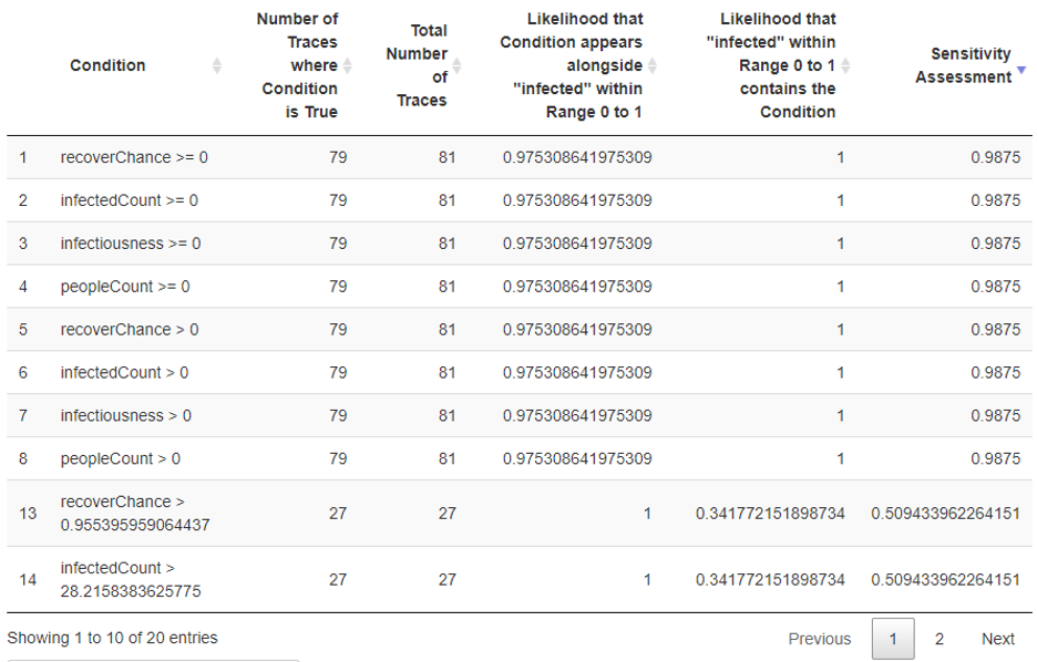
Figure 10: Sensitivity Assessment table
Getting HASH simulation outputs into the Sensitivity Assessor
VMASC is freely releasing its own-developed tooling for easily ingesting HASH simulation outputs within the Sensitivity Assessor. The process outlined below enables anybody to ingest HASH simulation data easily within the Sensitivity Assessor.
Step 1. obtain the JSON output of your simulation model
The JSON output of HASH simulation experiment runs can be downloaded within HASH Core or pulled directly from the generated JSON-State output in HASH Engine
Step 2. convert your output into a readable format
The Sensitivity Assessor expects data to be provided to it in a particular structure, and in CSV format. HASH simulation experiment run outputs can be converted for you into the expected format using VMASC's web-based HASH to Sensitivity Assessor utility.
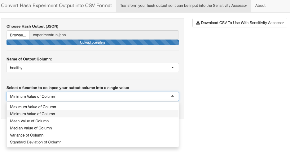
Figure 11: the HASH to Sensitivity Assessor utility
To use the HASH to Sensitivity Assessor:
- Upload HASH experiment JSON file using the Browse... button under Choose HASH Output (JSON)
- The variables from the uploaded file populate the Name of Output Column: selection box
- Select one variable from the Name of Output Column: selection box
- This is the variable to interest to gather insight into using the Sensitivity Assessor
- Use the Select a function to collapse your output column into a single value selection box. This is the function that will be used to transform the sequence of output values, specified in the Output Column, for each simulation run into a single value. The single value returned back is based on the function chosen. See below for more details:
- Every function that can be chosen is a many-to-one function. This means that it will take the entire column of values for a simulation run from the Output Column as input and return a single value back.
- This will result in a single value generated from each experiment, corresponding to a unique simRunId.
- Alternatively stated as: each variable's value is collected at each time step; therefore, this conversion process scans the time series to retrieve or generate one value based on the selected function.
- Click "Download CSV To Use With Sensitivity Assessor"
- Runs the tool using the selections from Steps 2 & 3 and generates a CSV file
- This file includes:
simRunId- variables names and their corresponding values used in the experiment
- selected output column name based on selection in Step 2 along with corresponding value based on the function selected in Step 3
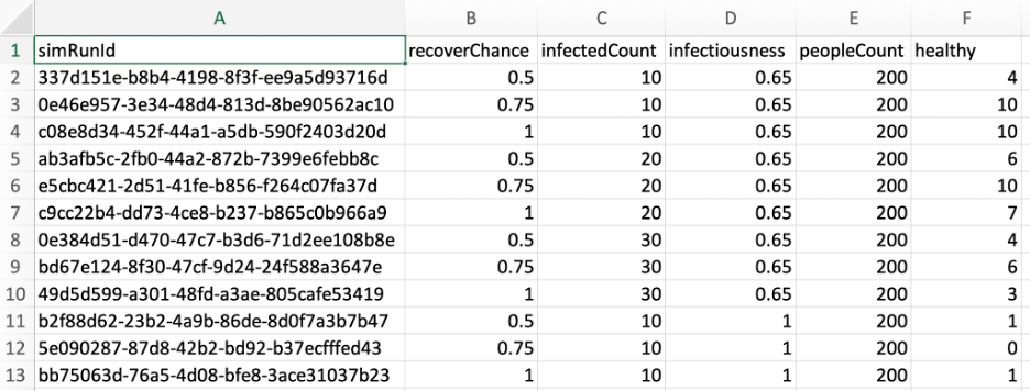
Figure 12: the CSV file corresponding to a HASH experiment JSON file generated by the HASH to Sensitivity Assessor utility
Step 3. upload the generated CSV file into the Sensitivity Assessor
By uploading the resultant .csv file generated by the HASH to Sensitivity Assessor tool into the Sensitivity Assessor itself you can now begin to analyze your HASH simulation experiment's outputs.
Case study: using the Sensitivity Assessor
Recall the original question we set out to answer earlier in this post: “How can we better understand and quantify the dynamics related to the input parameters in the simulation that contribute to simulation runs with no healthy people in the population at a point in time?”
To track down what may be causing this outcome of interest, we ran several experiments using HASH. The experiment created in HASH was a multiparameter value sweep, varying four different parameters with three different values in each. These parameters were:
recoverChance: the probability of an agent recovering after being infected with the virusinfectedPeople: the minimum number of infected agents at the beginning of the simulationinfectiousness: the basic reproductive number of the virus (R0), representing on average how many uninfected agents each agent infected with the virus will in turn infectpeopleCount: the total number of agents starting in the simulation
After the experiment run finished executing, we downloaded the output as JSON, and uploaded it into the HASH to Sensitivity Assessor web utility. To explore our research question, we selected the number of healthy people in the simulation run as the Output Column and used the “minimum” function to identify simulation runs with no healthy people in the simulated population at a point in time (see Figure 11). The CSV file produced was then loaded into the Sensitivity Assessor for analysis (see Figure 12).
Before beginning our work with the Sensitivity Assessor we formed a number of hypotheses as to what parameters might be contributing to simulation runs with no healthy people in the simulated population at a point in time. These included:
- The virus might have a very low chance of recovery resulting in agents staying sick for long periods of time; thus, resulting in zero healthy population at certain points during a simulation run.
- The virus might spread very rapidly when lots of agents are in the simulation. This mimics an urban setting where the population density is high causing infected agents to pass the virus on more quickly than in rural settings. This dynamic could create a situation where the virus quickly passed through the entire simulated population resulting in zero healthy agents at a certain point in time.
- The virus might be very infectious causing it to pass through the population quickly no matter how many (or how few) agents are in the simulation.
- Perhaps - independent of the chance of recovery from the virus or the infectiousness of the virus - if enough agents initially are infected, then the virus may pass very quickly to the few remaining healthy agents resulting in a simulation run. Thus, resulting in zero healthy agents at a certain point in time.
To identify which, if any, of these hypotheses were correct we applied the Sensitivity Assessor to generate a variety of predicates related to conditions in simulation runs that: (1) are true in runs where zero healthy individuals exist at a certain point in time and (2) are not true in simulation runs where at least one healthy individual exists at a certain point in time. The two predicates with the highest sensitivity assessments were:
infectiousness> 1.4: i.e., how many uninfected agents, on average, an infected agent will infectinfectedPeople> 28: i.e., the initial count of infected individuals
This enabled us to definitively identify what factors were contributing to runs within our HASH simulation model that contained zero healthy agents during portions of their runtime. A sufficiently high basic reproductive number of the virus along with more initial infectious agents would produce fewer areas of the landscape for healthy agents to move without risk of exposure to the virus. Agents' movement across the landscape randomly and under the identified conditions would result in the virus infecting most agents quickly. As a result, very few time steps in a simulation run under these parameters would be required for no healthy agents to remain. These results would occur independent of both the agent population size and the chance of recovery from the virus. In our trials we explored agent population sizes from 200 to 400 in size.
The takeaway message, under the assumptions present in this simulation, is that for a virus with a reproductive number greater than 1.4 (similar to that of influenza) minimizing the chance that those initially infected with the virus spread it to others is paramount. Otherwise, it is just a matter of time before there are very few and possibly no healthy folks to provide essential services.
It is important to note that while this explanation seems simple it does completely match any of our original hypotheses. Instead it involves two input parameters acting in combination, while two others do not contribute to the explanation. Researchers often are forced to spend an enormous amount of time and effort quantitatively demonstrating the dynamics that contribute to unanticipated outcomes. Even when they have a partially correct initial hypothesis about what is driving the outcome it can be painstaking to formally quantify the contribution of a condition or set of conditions on the output. By consuming HASH simulation model experiment run outputs, the Sensitivity Assessor helps facilitate this process and reduce the effort needed to gain insight into these types of outcomes.
The Sensitivity Assessor team
- Christopher J. Lynch, Ph.D. (Bio, X) leads the Data Analytics Working Group at VMASC of Old Dominion University. His research focuses on data analytics, simulation analytics, and health informatics. cjlynch@odu.edu
- Craig Jordan (Bio) is the PI and team lead for a project developing a series of simulation models to examine the impact of possible changes to the organ transplant ecosystem. cajordan@odu.edu
- Virginia Zamponi (LinkedIn) is a Graduate Research Assistant at VMASC and a Graduate Student in the Old Dominion University Computational Modeling and Simulation Engineering (CMSE) Department. vzamp001@odu.edu
- Kevin O’Brien (LinkedIn) is a Computer Systems Analyst at VMASC. His current work focuses on simulating systems and data analysis. kobrien@odu.edu
- Erik Jensen (Google Scholar) is a Graduate Research Assistant at VMASC and a Graduate Student in the Computational Modeling and Simulation Engineering (CMSE) Department of Old Dominion University. ejens005@odu.edu
About HASH
HASH is building the next generation of decision-making, data modeling, and knowledge management tools. Through an integrated global entity graph and rich simulations, HASH aims to enable everybody to make the right decisions.
Useful links
- VMASC Sensitivity Assessor
- VMASC HASH to Sensitivity Assessor conversion tool
- HASH Core simulation development, exploration and experimentation environment
- HASH Engine simulation engine
Get new posts in your inbox
Get notified when new long-reads and articles go live. Follow along as we dive deep into new tech, and share our experiences. No sales stuff.